cs180
Project 5: Fun With Diffusion Models
I switch between “I” and “we” as well as past and present tense in this website. Sorry!
Project 5A: The Power of Diffusion Models
Part 0: Setup
In this part, we used the DeepFloyd IF diffusion model, which is a two-stage model trained by Stability AI. We also used precomputed text embeddings to generate images. We used seed 88 for all parts.
We loaded stage 1 and stage 2 of the DeepFloyd model separately and generated images with each.
num_inference_steps=20


num_inference_steps=20
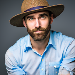

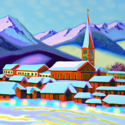
num_inference_steps=40
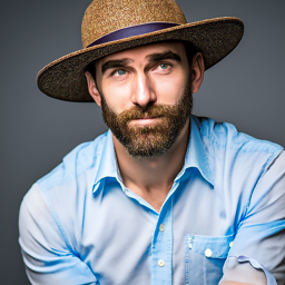

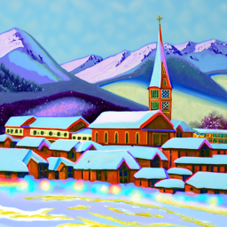
num_inference_steps=80
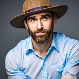

We can see that as we increase the number of inference steps, the images become more realistic and detailed. For instance, we can see more details in the wrinkles between the man’s eyebrows and in the UFOs in the background of the rocket ship image. All of the images seem faithful to the text prompts, but they just differ in the amount of fine detail that is present in the image, based on num_inference_steps.
Part 1.1: Implementing the Forward Process
We implemented the forward diffusion process in forward(im, t), defined by
We were given the \(\bar{\alpha}_t\) values for each \(t\), where \(\bar{\alpha}_t\) is close to 1 for small \(t\) (clean image) and close to 0 for large \(t\) (pure noise). We ran the forward process for t = 250, 500, 700.

Campanile

Noisy Campanile at t=250

Noisy Campanile at t=500

Noisy Campanile at t=750
Part 1.2: Classical Denoising
I used a Gaussian blur of kernel size 7 and sigma 2 to try to denoise these images classically.

Noisy Campanile at t=250

Noisy Campanile at t=500

Noisy Campanile at t=750

Gaussian blur denoising at t=250

Gaussian blur denoising at t=500

Gaussian blur denoising at t=750
Part 1.3: One-Step Denoising
We used the DeepFloyd stage 1 UNet to denoise the image by estimating the noise in the image and then removing it. We got the estimate of the clean image by rearranging the equation above to be an expression for \(x_0\) in terms of \(x_t\) (the noised image) and \(\epsilon\) (the estimated noise from the UNet output).

Original Campanile

Noisy Campanile at t=250

Noisy Campanile at t=500

Noisy Campanile at t=750

One-step denoising at t=250

One-step denoising at t=500

One-step denoising at t=750
Part 1.4: Iterative Denoising
The results were much better with one-step denoising compared to classical denoising, but the still performance degraded as more noise was added to the image. We used iterative denoising to address this issue. We created a list strided_timesteps of monotonically decreasing timesteps, starting at 990 and ending at 0 in 30 step increments. Thus, strided_timesteps[0] corresponded to pure noise, and strided_timesteps[-1] to the clean image. On the ith denoising step at t = strided_timesteps[i], we get to t' = strided_timesteps[i+1] (slightly less noisy) using the following formula:
The variables are defined in the spec. \(v_\sigma\) is random noise that we add via add_variance, defined for us in the starter code. We implemented the function iterative_denoise(image, i_start), where image is a noisy image and i_start is the index at which we start at in strided_timesteps (i.e. how noised the image is). We added noise to the image using t=strided_timesteps[10] and then ran iterative_denoise on the image using i_start=0 for the results below.

Noisy Campanile at t=90

Noisy Campanile at t=240

Noisy Campanile at t=390

Noisy Campanile at t=540

Noisy Campanile at t=690

Original Campanile

Iteratively denoised Campanile

One-step denoised Campanile

Gaussian blurred Campanile
Part 1.5: Diffusion Model Sampling
Now, we can generate images from scratch by setting i_start=0 in the call to iterative_denoise and passing in pure noise. This effectively denoises pure noise to create a new image. We did this on the prompt “a high quality photo”. Here are 5 sampled images.


Part 1.6: Classifier-Free Guidance (CFG)
To further improve performance, we implemented classifier-free guidance. In CFG, we compute both a conditional and unconditional noise estimate, which are denoted \(\epsilon_c\) and \(\epsilon_u\) respectively. The new noise estimate using CFG is then
\[\epsilon = \epsilon_u + \gamma (\epsilon_c - \epsilon_u)\]We use \(\gamma = 7\), and we use an empty prompt "" for unconditional guidance.
Here are images generated using CFG.


Part 1.7: Image-to-image Translation
To make edits to existing images, we can take a real image, add noise to it, and then denoise it, following the SDEdit algorithm. The more noise we add, the more the model can be “creative” and generate something new (not in the original image). We use the noise levels [1, 3, 5, 7, 10, 20], so we add noise using forward(im, strided_timesteps[i_start]) and we denoise by passing in the appropriate i_start to iterative_denoise_cfg.
I did this process on the Campanile image, as well as images of a dog and a tree.

SDEdit with i_start=1

SDEdit with i_start=3

SDEdit with i_start=5

SDEdit with i_start=7

SDEdit with i_start=10

SDEdit with i_start=20

Campanile

SDEdit with i_start=1

SDEdit with i_start=3

SDEdit with i_start=5

SDEdit with i_start=7

SDEdit with i_start=10

SDEdit with i_start=20

Dog

SDEdit with i_start=1

SDEdit with i_start=3

SDEdit with i_start=5

SDEdit with i_start=7

SDEdit with i_start=10

SDEdit with i_start=20

Tree
Part 1.7.1: Editing Hand-Drawn and Web Images
We experimented with hand-drawn and other non-realistic images using our diffusion model. We followed the same process as described above, using noise levels [1, 3, 5, 7, 10, 20] to noise and denoise images.
I did this on an image of tree clip art, as well as my hand-drawn images of an apple and the sky. The yellow-ish circle in the sky image is supposed to be the Sun, although I don’t think it came across very well after the code compressed my hand-drawn image.

SDEdit with i_start=1

SDEdit with i_start=3

SDEdit with i_start=5

SDEdit with i_start=7

SDEdit with i_start=10

SDEdit with i_start=20

Tree Clip Art

SDEdit with i_start=1

SDEdit with i_start=3

SDEdit with i_start=5

SDEdit with i_start=7

SDEdit with i_start=10

SDEdit with i_start=20

Hand-Drawn Apple

SDEdit with i_start=1

SDEdit with i_start=3

SDEdit with i_start=5

SDEdit with i_start=7

SDEdit with i_start=10

SDEdit with i_start=20

Hand-Drawn Sky
Part 1.7.2: Inpainting
We can use our model to inpaint, where we mask out one part of an image and use the model to fill it in. Given an image x_orig and a binary mask m, we can create a new image that has the same content where m is 0 and new content wherever m is 1. We run the diffusion denoising loop, but after every step, we “force” x_t to have the same pixels as x_orig where m is 0:
I inpainted the top of the campanile, as well as a photo of my brother and the Seattle Space Needle.

Campanile

Mask

Hole to fill

Campanile inpainted

Brother

Mask

Hole to fill

Brother inpainted

Space needle

Mask

Hole to fill

Space needle inpainted
Part 1.7.3: Text-Conditional Image-to-image Translation
We followed the procedure described in part 1.7, but we changed the prompt to be one of the precomputed prompts instead of “a high quality photo”. This makes the image look more like the text prompt at higher noise levels (since the model can be more creative when there is more noise).
Here is the text prompt “a rocket ship” and the Campanile image.

Rocket ship at noise level 1

Rocket ship at noise level 3

Rocket ship at noise level 5

Rocket ship at noise level 7

Rocket ship at noise level 10

Rocket ship at noise level 20

Campanile
Here is the text prompt “a photo of a dog” and a squirrel image.

A photo of a dog at noise level 1

A photo of a dog at noise level 3

A photo of a dog at noise level 5

A photo of a dog at noise level 7

A photo of a dog at noise level 10

A photo of a dog at noise level 20

Squirrel
Here is the text prompt “a photo of a man” and a tree image.

A photo of a man at noise level 1

A photo of a man at noise level 3

A photo of a man at noise level 5

A photo of a man at noise level 7

A photo of a man at noise level 10

A photo of a man at noise level 20

Tree
Part 1.8: Visual Anagrams
We denoise an image at step t normally using one prompt to get noise estimate \(\epsilon_1\). At the same time, and we flip the image upside down and denoise it using another prompt to get noise estimate \(\epsilon_2\). We then flip \(\epsilon_2\) back so it is right-side up, and we average the two noise estimates. We then perform a denoising diffusion step with the averaged noise estimate.
We implemented the algorithm as described in the spec.
Here is an anagram from the prompts 'an oil painting of an old man' and 'an oil painting of people around a campfire'.

An oil painting of an old man

An oil painting of people around a campfire
Here is an anagram from the prompts 'a photo of a dog' and 'a photo of a man'.

A photo of a dog

A photo of a man
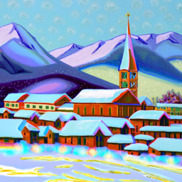
Here is an anagram from the prompts 'an oil painting of a snowy mountain village' and 'an oil painting of people around a campfire'.

An oil painting of a snowy mountain village

An oil painting of people around a campfire
Part 1.9: Hybrid Images
We can create hybrid images by combining the low and high frequencies of two different noise estimates from different text prompts. We denoise an image at step t using one prompt to get noise estimate \(\epsilon_1\) and using another prompt to get noise estimate \(\epsilon_2\). Then, we get the combined noise estimate using \(f_{\text{lowpass}}(\epsilon_1) + f_{\text{highpass}}(\epsilon_2)\).
Here is the hybrid image from the prompts “a lithograph of a skull” (low pass) and “a lithograph of waterfalls” (high pass).


Here is the hybrid image from the prompts “a lithograph of a skull” (low pass) and “a lithograph of houseplants” (high pass).


Here is the hybrid image from the prompts “a lithograph of a panda” (low pass) and “a lithograph of houseplants” (high pass).


Project 5B: Diffusion Models from Scratch
Part 1: Training a Single-Step Denoising UNet
We implemented the Single-Step Denoising UNet as specified by the process described in Part 1.1 of the project spec.
To train this denoiser, we need to generate training data pairs of \((z, x)\) where each \(x\) is a clean MNIST digit and \(z\) is a noised version. We use the following:
\[z = x + \sigma \epsilon, \epsilon \sim \mathcal{N}(0, 1)\]Here is a visualization of the noising processes over \(\sigma = [0.1, 0.2, 0.4, 0.5, 0.6, 0.8, 1.0]\), with normalized \(x \in [0, 1]\). Each column corresponds to a sigma value in the list, in the order they are listed.
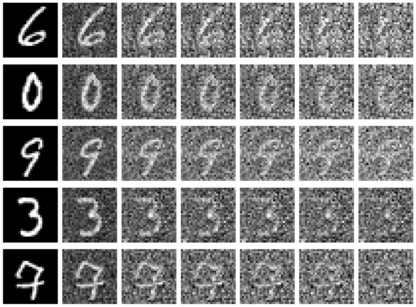
I trained the UNet to denoise noisy image \(z\) with \(\sigma = 0.5\) applied to clean image \(x\). I used batch size 256, hidden dimension D = 128, and Adam optimizer with learning rate 1e-4. I trained for 5 epochs. I used L2 loss between the denoised image output from the UNet and the clean image \(x\).
Here is the graph of training losses.
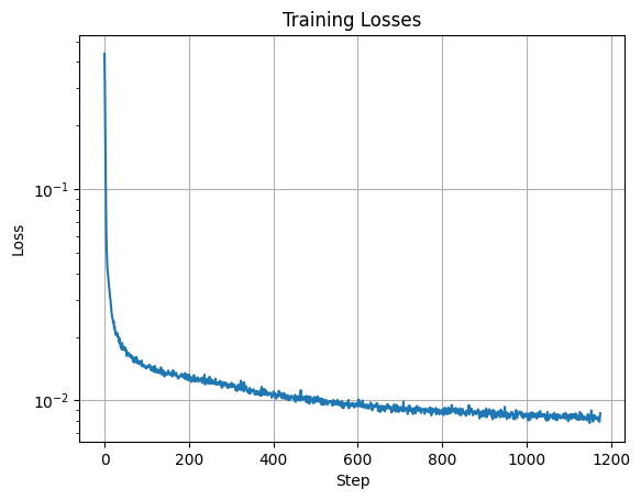
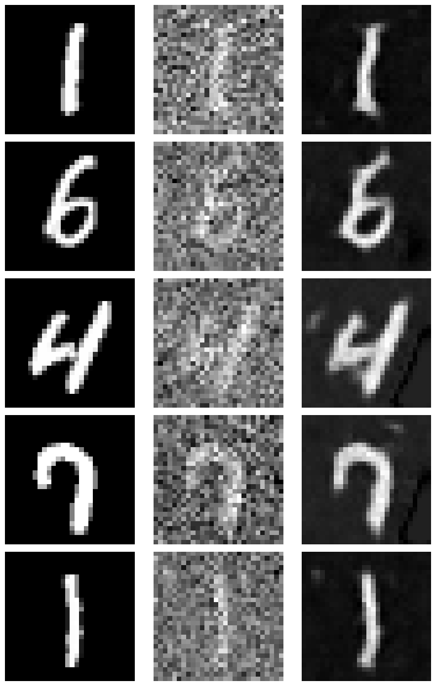
Here are sample results on the test set after the 1st epoch of training. The first column is the original clean image, the second column is the noisy image using \(\sigma=0.5\), and the third column is the model output from denoising the noisy image.
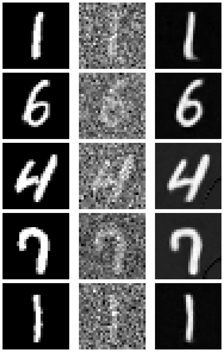
Here are sample results on the test set after the 5th epoch of training. Again, the first column is the original clean image, the second column is the noisy image using \(\sigma=0.5\), and the third column is the model output from denoising the noisy image.
We tested the model on MNIST images that were noised with different \(\sigma\) values to see how well it performed on out-of-distribution data. Here are the results for \(\sigma = [0.0, 0.2, 0.4, 0.5, 0.6, 0.8, 1.0]\)

Part 2: Training a Diffusion Model
Time Conditioning
We implemented the UNet with time conditioning according to the details and architecture specified in the project spec. Instead of a separate UNet for each timestep, we trained a model to be conditioned on the timestep. We added fully connected blocks for embedding the timestep into the up-layers of the UNet.
This model predicts a noise estimate rather than the denoised image directly. We use L2 loss over the predicted noise using the model and the actual noise added to the image.
Now, we noise images using the following formula:
\[x_t = \sqrt{\bar{\alpha}_t} x_0 + \sqrt{1 - \bar{\alpha}_t} \epsilon, \epsilon \sim \mathcal{N}(0, 1)\]We want \(x_t\) at \(t=0\) to be the clean image and \(x_t\) at \(t=T\) to be pure noise. We create the beta, alpha_t, and alpha_t_bar lists as described in the spec. We use \(T=300\) as the total number of timesteps.
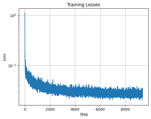
We trained the model \(\epsilon_\theta (x_t, t)\) to predict the noise in \(x_t\) given a noisy image \(x_t\) and timestep \(t\). We used batch size 128, hidden dimension D = 64, and Adam optimizer with initial learning rate of 1e-3. We also used an exponential learning rate decay scheduler with gamma \(0.1^{1/\text{num_epochs}}\). We trained for 20 epochs. We normalized \(t\) before passing it into the forward pass of the UNet.
Here is the training loss curve.
Here are the sampling results from the time-conditional UNet at epochs 5, 10, and 20.
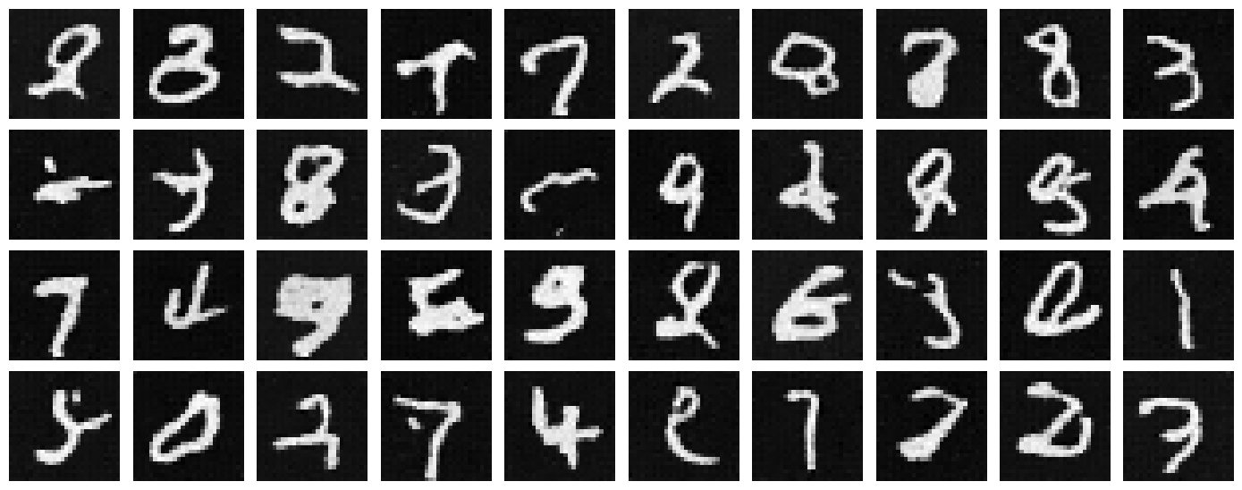
Epoch 5
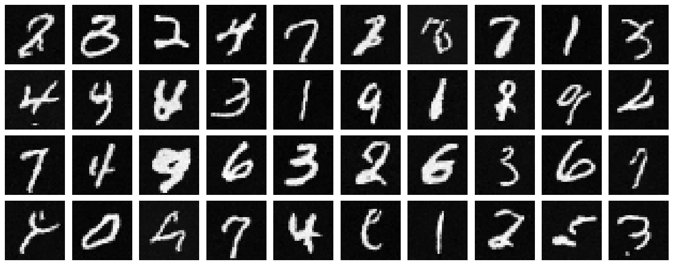
Epoch 10
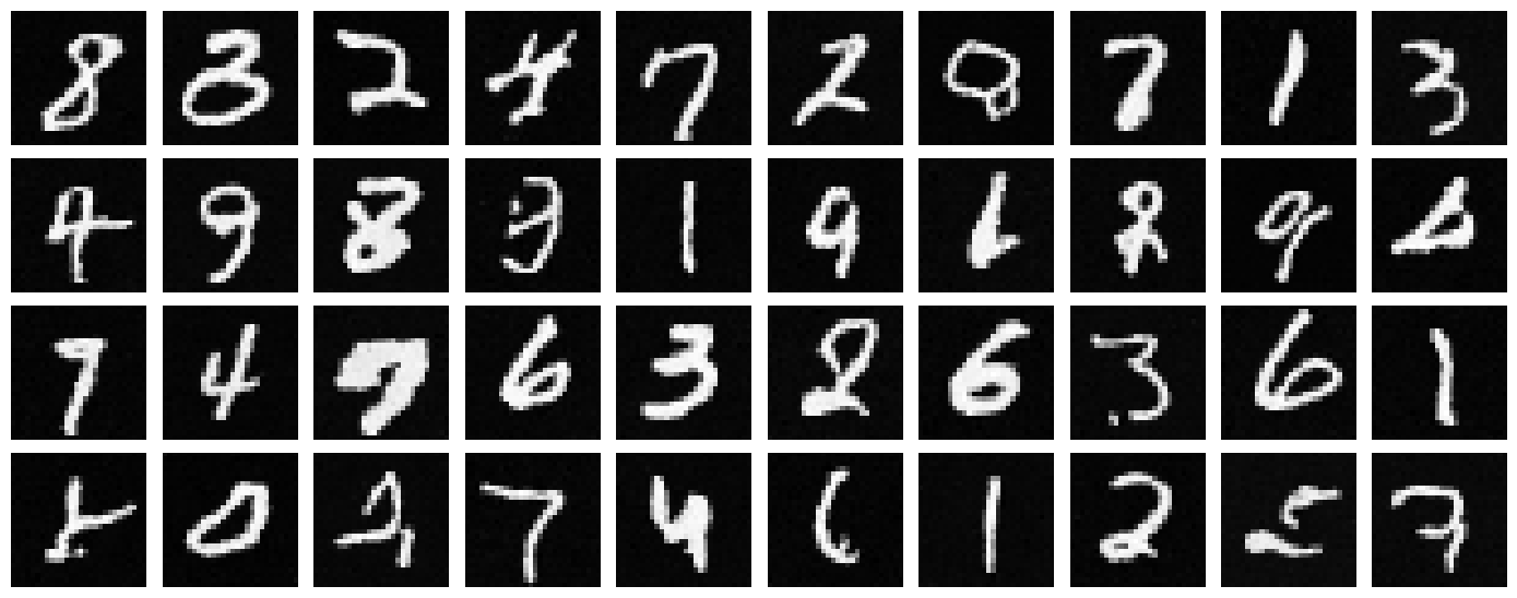
Epoch 20
Class Conditioning
To improve performance, we also condition the UNet on the class of the digit 0-9. To do this, we add two more fully connected blocks to the UNet architecture that take in a one-hot vector for the class of the digit. Because we still want the model to work without class conditioning, we use a mask such that 10% of the time, we drop the class conditioning vector by setting it to 0. For training this model, we use the same hyperparameters and learning rate scheduler as in the time conditioning case. We implement the class conditioning by following the procedure specified in the project spec.
Here is the training loss curve for the class conditional model.
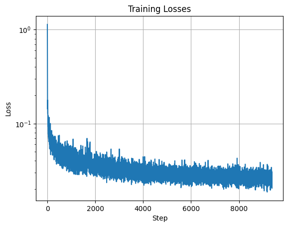
Here are the sampling results from the class-conditional UNet at epochs 5 and 20.
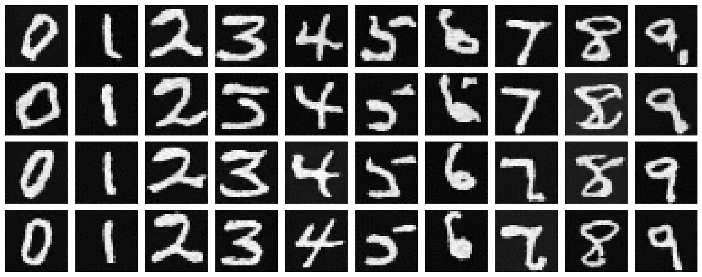
Epoch 5
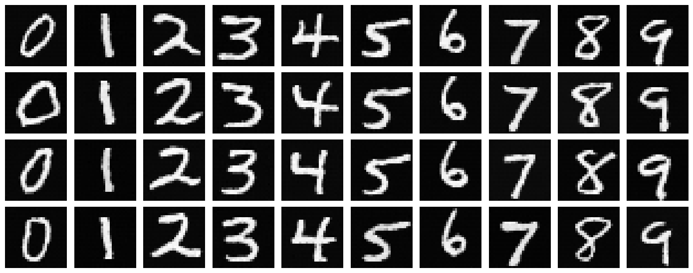
Epoch 20